COVID Crime Impacts
Posted on May 2, 2020 | 6 minute readCuriosity
I’ve been thinking a lot lately about what’s different now. When the lockdown first started, I couldn’t stop thinking about how government, specifically local government, was going to have to come up with solutions to new problems on the fly and try as much as possible to limit negative unintended consequences. I still am thinking about that a lot but I have definitely found myself considering more and more what it would be like to be faced with analytic questions in the middle of all of this in local government. And I don’t mean the brainstorming type of questions, I mean the Police Chief just walked into your office and asked you to take a look at the data and tell her exactly what is different. Sure we have our instincts and experience but is there anything in the data right now that might be useful?
Considering you have access to data (which is still a major problem for a lot of local governments out there), I think this would be a really exciting question to explore. Let’s take a quick crack at how someone might approach this question in a quick way to generate some insights. We may walk away with more questions than answers but that is generally the fun of it!
The Data
I am going to go with a dataset that I know is fairly robust just to make sure I have something good to play around with. I’m pulling down Police Department Calls for Service from the City of San Francisco’s open data portal. There is an R package interface to these Socrata data portals but I just downloaded to .csv to make things simple.
Let’s load the data really quick and take a look.
sf_crime <- read_csv("data/Police_Department_Calls_for_Service.csv")

str(sf_crime)
## tibble [3,340,360 × 14] (S3: spec_tbl_df/tbl_df/tbl/data.frame)
## $ Crime Id : num [1:3340360] 1.9e+08 1.9e+08 1.9e+08 1.9e+08 1.9e+08 ...
## $ Original Crime Type Name: chr [1:3340360] "Noise Nuisance" "Stolen Vehicle" "Fight No Weapon" "Well Being Check" ...
## $ Report Date : chr [1:3340360] "01/01/2019" "01/05/2019" "01/07/2019" "01/25/2019" ...
## $ Call Date : chr [1:3340360] "01/01/2019" "01/05/2019" "01/07/2019" "01/25/2019" ...
## $ Offense Date : chr [1:3340360] "01/01/2019" "01/05/2019" "01/07/2019" "01/25/2019" ...
## $ Call Time : 'hms' num [1:3340360] 01:32:00 18:31:00 15:27:00 19:51:00 ...
## ..- attr(*, "units")= chr "secs"
## $ Call Date Time : chr [1:3340360] "01/01/2019 01:32:00 AM" "01/05/2019 06:31:00 PM" "01/07/2019 03:27:00 PM" "01/25/2019 07:51:00 PM" ...
## $ Disposition : chr [1:3340360] "ADV" "REP" "UTL" "HAN" ...
## $ Address : chr [1:3340360] "400 Block Of 2nd Av" "28th Av/balboa St" "400 Block Of Bush St" "Paul Av/carr St" ...
## $ City : chr [1:3340360] "San Francisco" "San Francisco" "San Francisco" "San Francisco" ...
## $ State : chr [1:3340360] "CA" "CA" "CA" "CA" ...
## $ Agency Id : num [1:3340360] 1 1 1 1 1 1 1 1 1 1 ...
## $ Address Type : chr [1:3340360] "Premise Address" "Intersection" "Premise Address" "Intersection" ...
## $ Common Location : chr [1:3340360] NA NA NA NA ...
## - attr(*, "spec")=
## .. cols(
## .. `Crime Id` = col_double(),
## .. `Original Crime Type Name` = col_character(),
## .. `Report Date` = col_character(),
## .. `Call Date` = col_character(),
## .. `Offense Date` = col_character(),
## .. `Call Time` = col_time(format = ""),
## .. `Call Date Time` = col_character(),
## .. Disposition = col_character(),
## .. Address = col_character(),
## .. City = col_character(),
## .. State = col_character(),
## .. `Agency Id` = col_double(),
## .. `Address Type` = col_character(),
## .. `Common Location` = col_character()
## .. )Very nice! Over three million records but it definitely needs a little massaging. I’m thinking that I want to be able to create comparison cohorts for the available years to see if I can isolate any differences to think more critically about. To do that, I’m going to need to do some work on my time variables. Let’s see what we can do!
sf_crime_clean <- sf_crime %>%
  janitor::clean_names() %>%
  mutate(report_date = as.POSIXct(call_date, format = "%m/%d/%Y")) %>%
  mutate(doy = yday(report_date)) %>%
  filter(doy <= yday(Sys.Date())) %>%
  mutate(report_year = year(report_date))
Now we can check this out really quick to see what it gave us.
sf_crime_clean %>%
  group_by(report_year) %>%
  count(name = "report_count") %>%
  ungroup() %>%
  ggplot(aes(report_year, report_count)) +
  geom_col(fill = "#133140") +
  geom_label(aes(label = scales::comma(report_count)), nudge_y = -20000) +
  scale_y_continuous(labels = scales::comma_format()) +
  jason_theme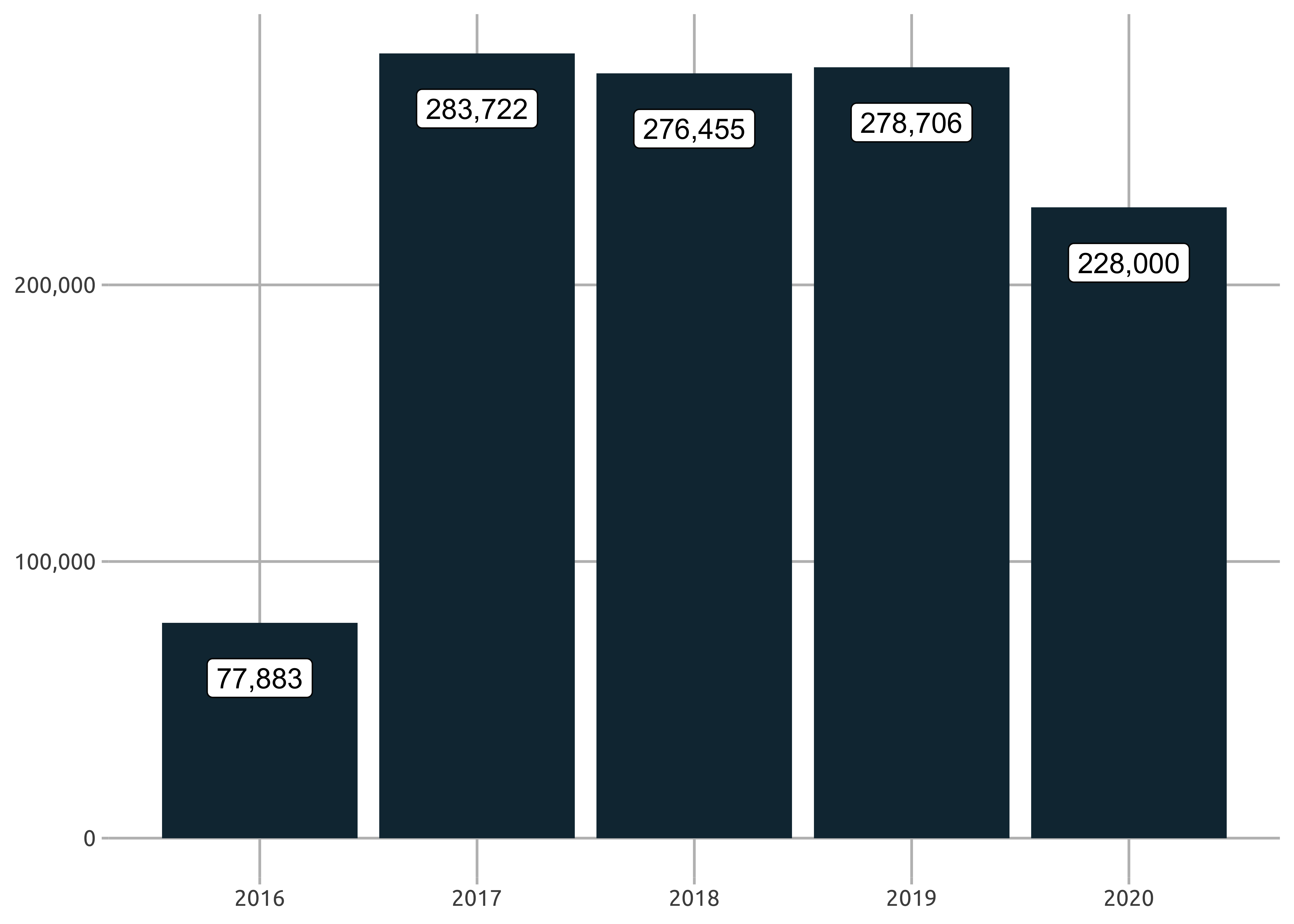
Great! I think I will choose to discard 2016 from now on. Looks like an incomplete year.
Let’s look at some differences in calls by year and description. I’m not being super analytic here, just scraping the surface for some high-level differences.
sf_crime_clean %>%
  filter(report_year != 2016) %>%
  group_by(report_year, original_crime_type_name) %>%
  count(name = "report_count") %>%
  ungroup() %>%
  pivot_wider(names_from = report_year, values_from = report_count) %>%
  mutate_at(.vars = vars(2:4), .funs = ~`2020` - .) %>%
  pivot_longer(cols = 2:5, names_to = "report_year", values_to = "report_count") %>%
  arrange(report_count) %>%
  head(n = 10)
## # A tibble: 10 x 3
## original_crime_type_name report_year report_count
## <chr> <chr> <int>
## 1 Traffic Stop 2017 -22589
## 2 Traffic Stop 2018 -15112
## 3 Homeless Complaint 2018 -10802
## 4 Traffic Stop 2019 -8591
## 5 Homeless Complaint 2017 -7582
## 6 22500e 2018 -6636
## 7 Muni Inspection 2018 -6303
## 8 22500e 2017 -6254
## 9 Suspicious Person 2017 -5466
## 10 Suspicious Person 2018 -5149Ok - I think I am going to choose to isolate Traffic Stop, Homeless Complaint, and Suspicious Person.
of_interest <- c("Traffic Stop", "Homeless Complaint", "Suspicious Person")

sf_crime_clean <- sf_crime_clean %>%
  filter(report_year != 2016) %>%
  filter(original_crime_type_name %in% of_interest)
Now maybe we should make a quick plot just to take a look at all three together.
sf_crime_clean %>%
  group_by(report_year, doy, original_crime_type_name) %>%
  count(name = "report_count") %>%
  ggplot(aes(doy, report_count, color = as.character(report_year))) +
  geom_line(color = "#133140") +
  facet_wrap(~original_crime_type_name) +
  gghighlight(report_year == 2020, calculate_per_facet = TRUE) +
  geom_vline(xintercept = 75, color = "black") +
  jason_theme +
  theme(strip.background = element_rect(fill = "#133140"),
        strip.text = element_text(color = "white", face = "bold", size = 12))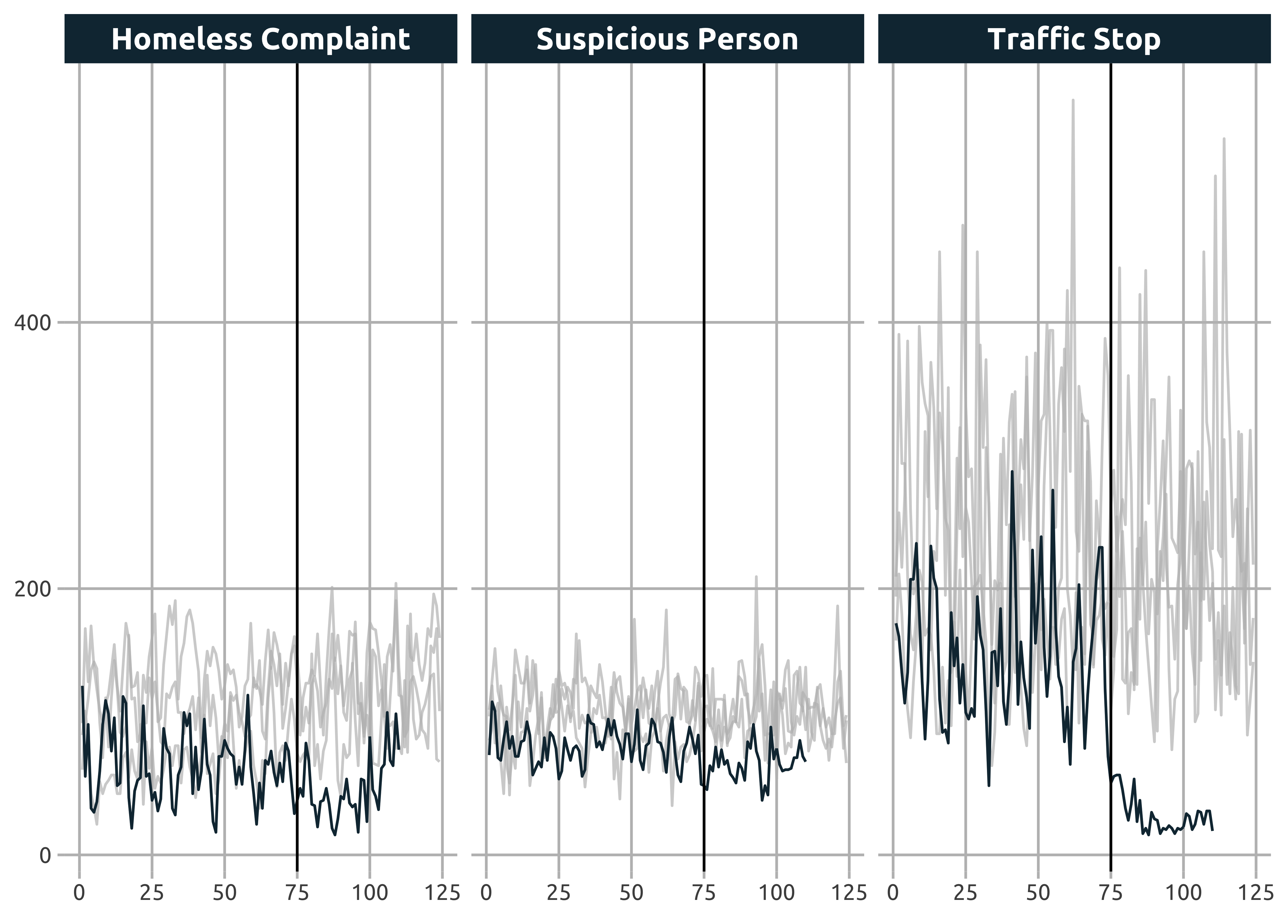
Wow! All three look like they are down for this period of the year but Traffic Stops appear to be significantly impacted!
Quick check of trend differences now.
sf_crime_clean %>%
  filter(original_crime_type_name == "Traffic Stop") %>%
  group_by(report_year, doy, original_crime_type_name) %>%
  count(name = "report_count") %>%
  ungroup() %>%
  ggplot(aes(doy, report_count, group = as.character(report_year))) +
  geom_line(color = "#133140") +
  geom_smooth(se = F, method = "lm", color = "#133140") +
  gghighlight(report_year == 2020, calculate_per_facet = TRUE) +
  geom_vline(xintercept = 75, color = "black") +
  jason_theme +
  theme(strip.background = element_rect(fill = "#133140"),
        strip.text = element_text(color = "white", face = "bold", size = 12))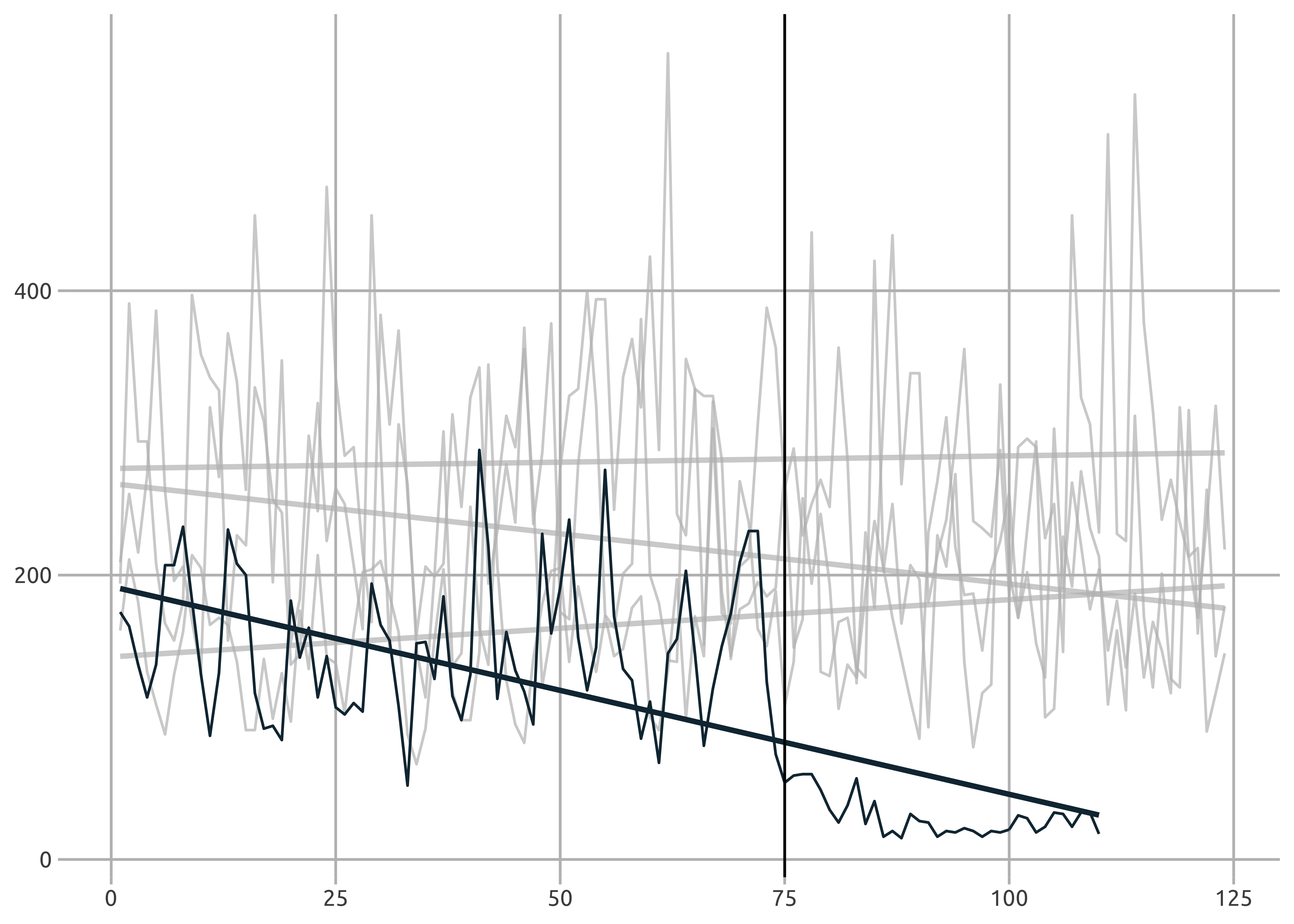
And for the final plot, I’m giving Dr. Ken Steif’s recommendation a try. I’m interested in seeing not only differences by year, but differences pre and post COVID-19 lockdown.
sf_crime_clean %>%
  filter(original_crime_type_name == "Traffic Stop") %>%
  group_by(report_year, doy, original_crime_type_name) %>%
  count(name = "report_count") %>%
  ungroup() %>%
  mutate(covid_test = doy < 75) %>%
  ggplot(aes(doy, report_count, group = interaction(covid_test, report_year))) +
  geom_line(color = "#133140") +
  geom_smooth(se = F, method = "lm", color = "#133140") +
  gghighlight(report_year == 2020) +
  geom_vline(xintercept = 75, color = "black") +
  labs(title = expression(paste(bold("San Francisco Open Data: "), "Police Calls for Service")),
       subtitle = "Difference in Traffic Stops by year, pre and post COVID lockdown. Prior years\nin grey and current year (2020) is highlighted.", caption = "Source: https://datasf.org/opendata/\nAuthor: Jason Jones") +
  jason_theme +
  theme(strip.background = element_rect(fill = "#133140"),
        strip.text = element_text(color = "white", face = "bold", size = 12))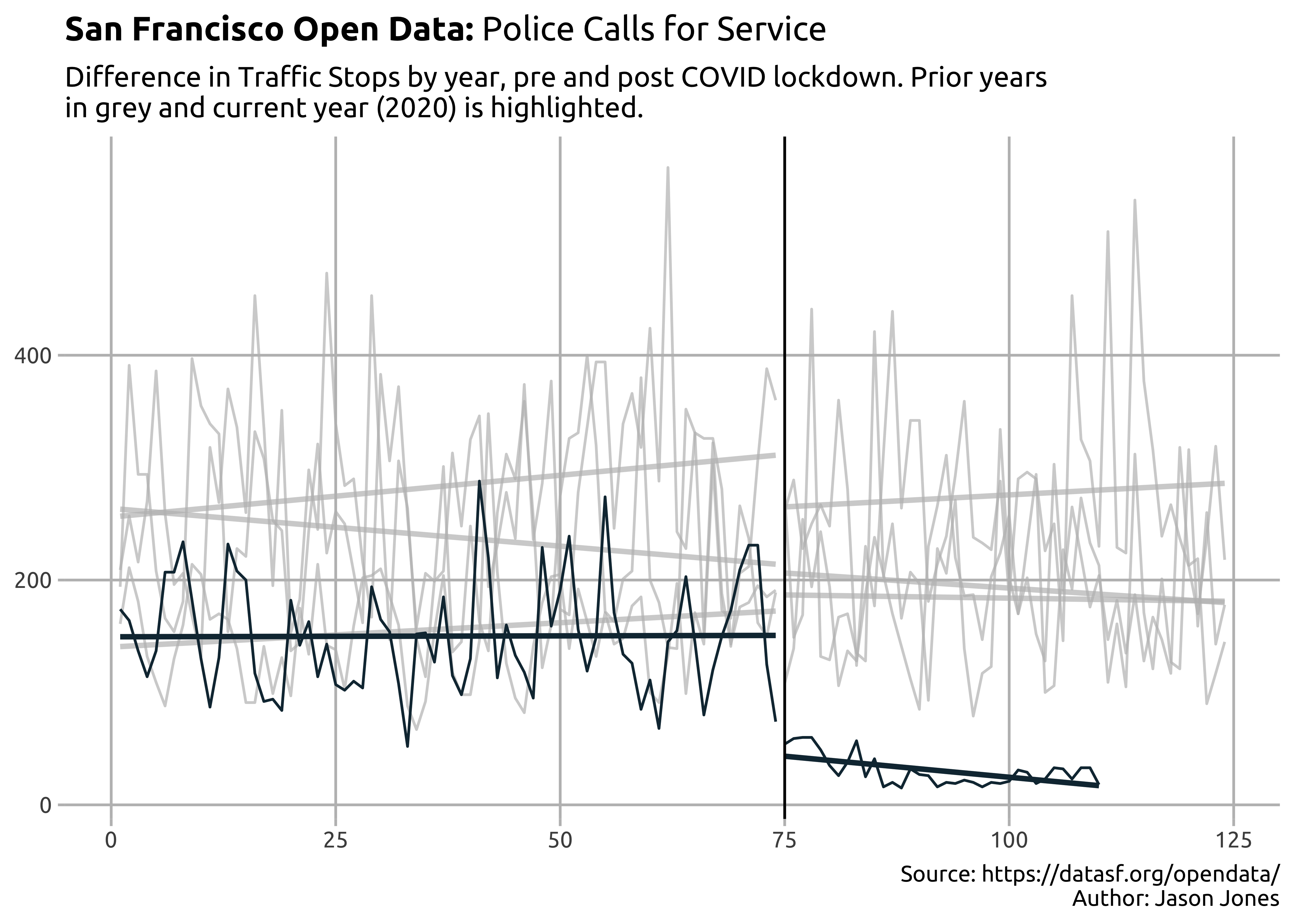
Tags:R Markdown
	  R
	  crime
	  tidyverse
	  open data
comments powered by Disqus