Weather Data
Posted on May 29, 2019 | 3 minute readThe Boring Bits
# Load packages ----
library(tidyverse)
library(tigris)
library(sf)
library(riem)
library(kableExtra)
Finding Home
Let’s start by grabbing the Chapel Hill boundary and then doing a test plot.
# Retrieve Chapel Hill boundary ----
chapel_hill <- places(state = 37, year = 2017) %>%
  st_as_sf() %>%
  filter(NAME == "Chapel Hill")
chapel_hill %>%
ggplot() +
geom_sf(fill = NA, color = "Red") +
theme(panel.background = element_blank())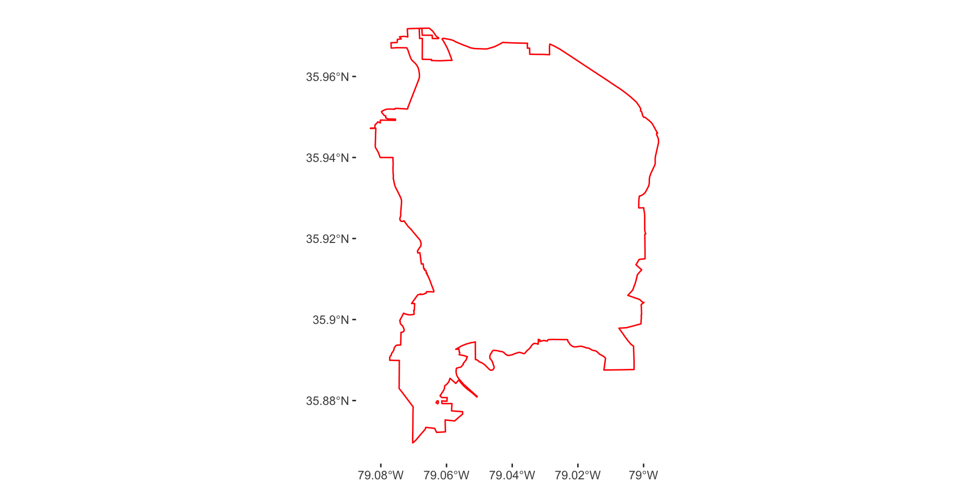
Weather Stations
Now we need to grab all of the weather stations for NC and do another test plot to make sure everything is working. We should see a nice collection of dots that looks like North Carolina!
# Retrieve weather stations ----
stations <- riem_stations(network = "NC_ASOS") %>%
  st_as_sf(coords = c("lon", "lat"), crs = st_crs(chapel_hill))

stations %>%
  ggplot() +
  geom_sf() +
  theme(panel.background = element_blank())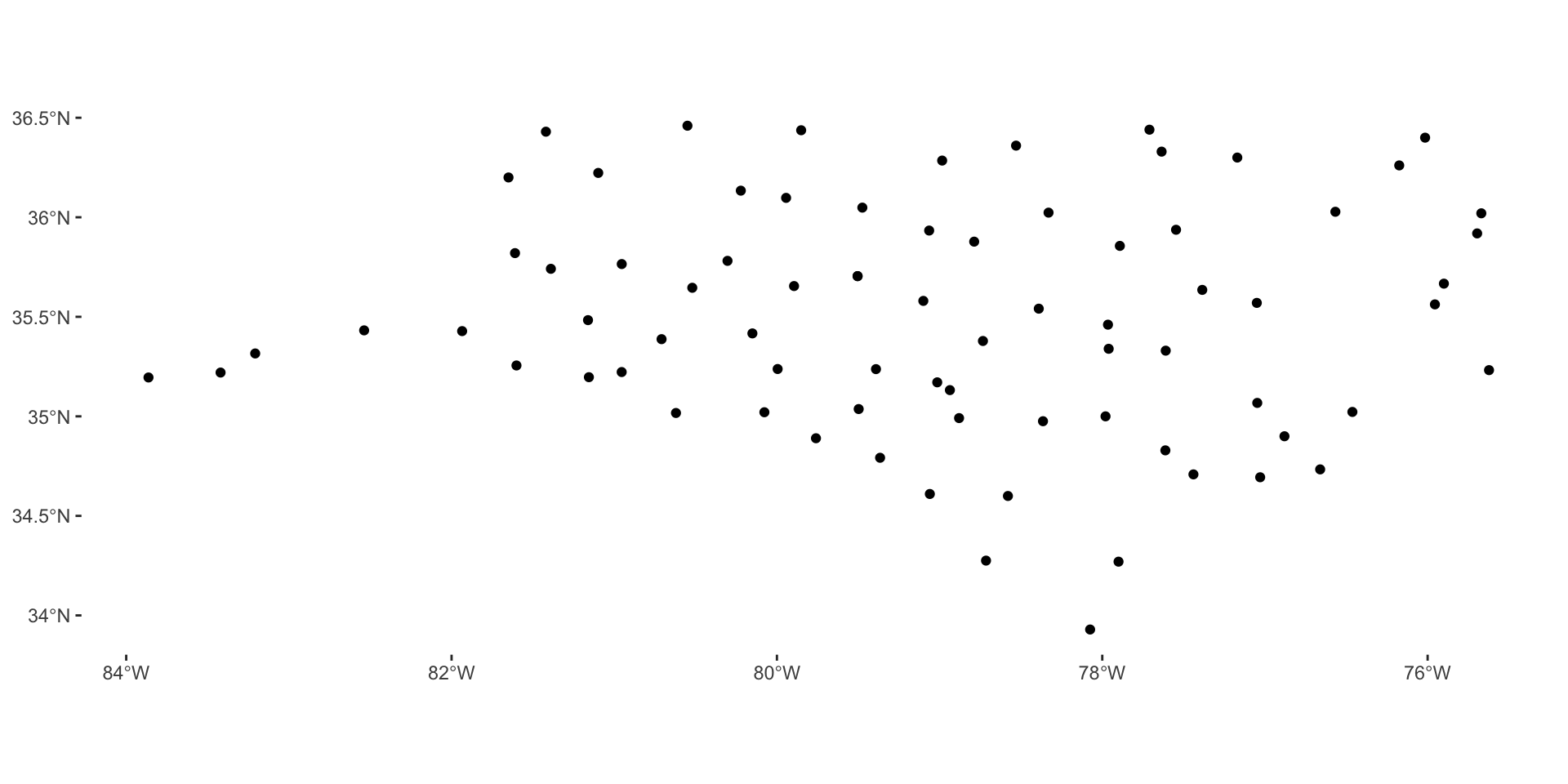
Subset Chapel Hill
Getting fancy now! We will do some geoprocessing to select only the weather station(s) that fall within the Chapel Hill boundary we grabbed first. A test plot should confirm that this worked for us.
# Select station in Chapel Hill ---
selection <- st_intersection(stations, chapel_hill)

# Confirm location ----
stations %>%
  filter(id == "IGX") %>%
  ggplot() +
  geom_sf(data = chapel_hill, fill = NA, color = "Red") +
  geom_sf() +
  theme(panel.background = element_blank())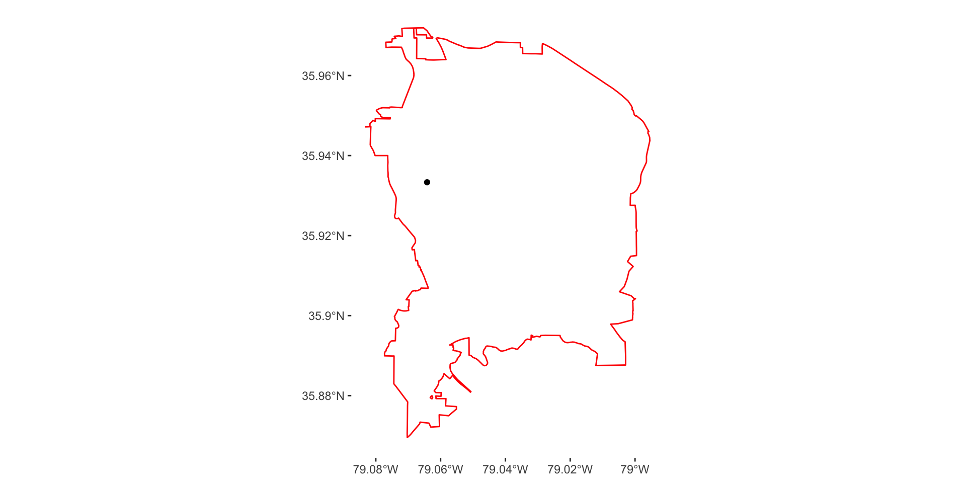
Retrieve Weather Data
Now that we know what weather station we want to focus on, we can retrive all of the data for that station.
# Retrieve weather data for station IGX ----
weather_dat <- riem_measures(station = "IGX")
UH-OH! Data shows that readings stopped in April 2018. A quick Google search revealed that the airport was actually closed in May 2018! Looks like we will need to try something else!
Next Closest Station
Maybe we can do some more geoprocessing and find the next closest station. Let’s start with that and then check out the results.
# Compute distances of stations from Chapel Hill center
stations <- chapel_hill %>%
  st_centroid() %>%
  st_distance(stations, by_element = TRUE) %>%
  as.integer %>%
  cbind(stations) %>%
  rename(distance = ".")

# Check out the results
stations %>%
  as_tibble() %>%
  select(-geometry) %>%
  top_n(-3, distance) %>%
  arrange(distance) %>%
  kable(col.names = c("Distance", "Station ID", "Name")) %>%
kable_styling()| Distance | Station ID | Name |
|---|---|---|
| 2384 | IGX | WILLIAMS_AIRPORT_(ASOS) |
| 23351 | RDU | RALEIGH-DURHAM_(ASOS) |
| 38880 | TTA | SANFORD-LEE_COUNTY_RGNL_AIRPORT |
Weather Data One More Time
Looks like RDU is the next closest weather station to the center of Chapel Hill. Let’s go get the weather data for that station now.
# Retrieve weather data again ----
weather_dat <- riem_measures(station = "RDU")
Awesome stuff! Now we can play around with the weather data a bit.
Monthly Average Temperature
weather_dat %>%
  filter(is.na(tmpf) != TRUE) %>%
  mutate(valid = lubridate::floor_date(valid, unit = "month")) %>%
  group_by(valid) %>%
  summarise(avg_temp = mean(tmpf)) %>%
  ungroup() %>%
  ggplot(aes(valid, avg_temp)) +
  geom_line(color = "#112E51") +
  geom_point(size = 3, color = "#FF7043") +
  labs(x = NULL, y = NULL) +
  theme(panel.background = element_blank())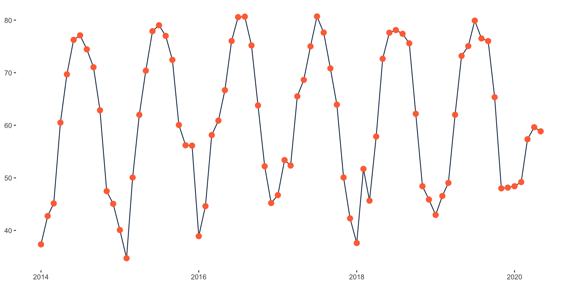
Daily Highs and Lows
highs <- weather_dat %>%
  filter(is.na(tmpf) != TRUE) %>%
  mutate(valid = lubridate::floor_date(valid, unit = "day")) %>%
  group_by(valid) %>%
  top_n(1, tmpf) %>%
  summarise(high = mean(tmpf)) %>%
  ungroup()

lows <- weather_dat %>%
  filter(is.na(tmpf) != TRUE) %>%
  mutate(valid = lubridate::floor_date(valid, unit = "day")) %>%
  group_by(valid) %>%
  top_n(-1, tmpf) %>%
  summarise(low = mean(tmpf)) %>%
  ungroup()

highs %>%
  left_join(lows, by = "valid") %>%
  gather("key", "value", 2:3) %>%
  ggplot(aes(valid, value, color = key)) +
  geom_line() +
  labs(x = NULL, y = NULL) +
  scale_color_manual(name = "Categories", values = c("#112E51", "#FF7043")) +
  theme(panel.background = element_blank())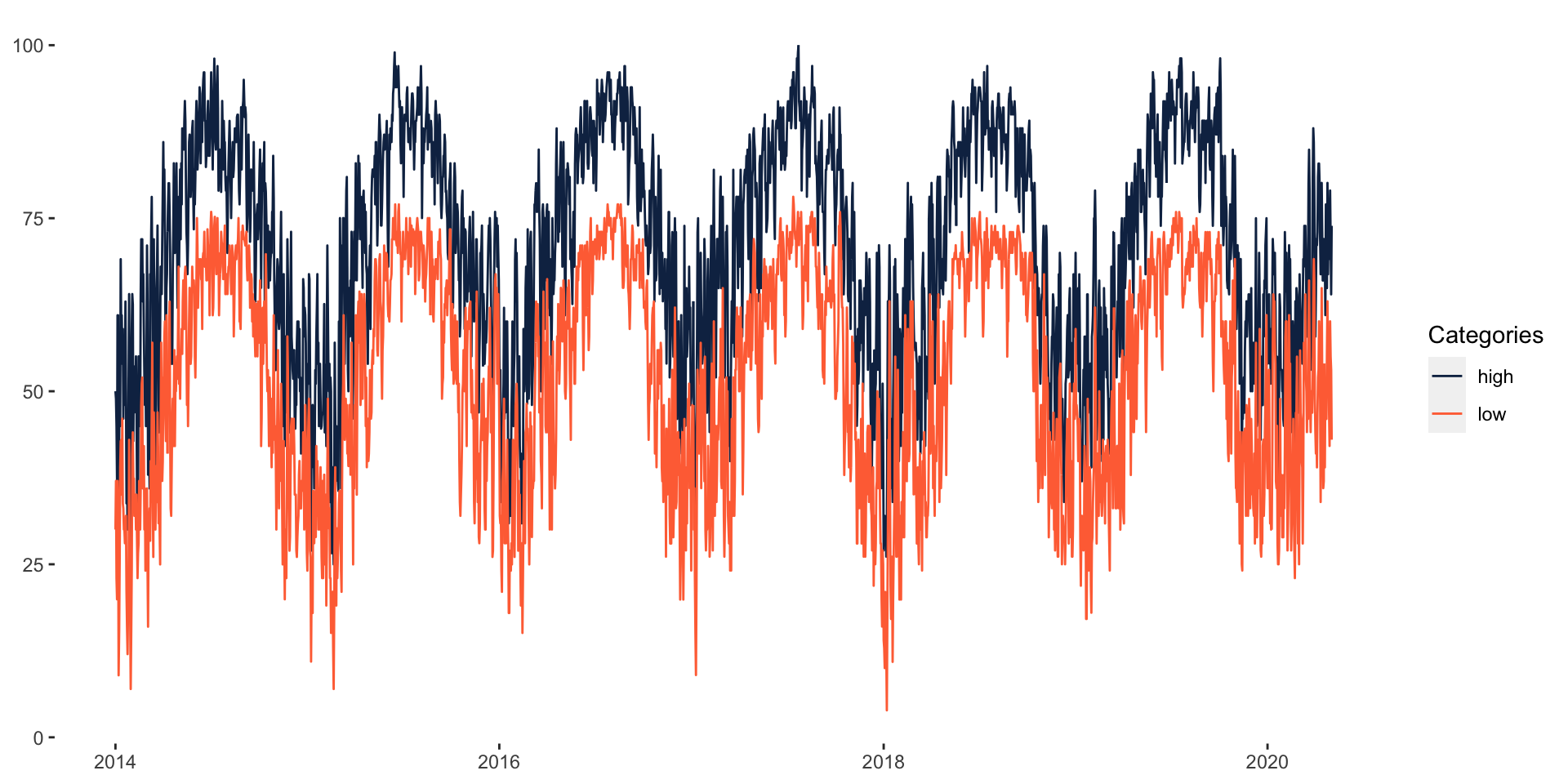
High and Low Differences, Monthly Variance
highs %>%
  left_join(lows, by = "valid") %>%
  mutate(diff = high - low) %>%
  mutate(valid = lubridate::floor_date(valid, unit = "month")) %>%
  group_by(valid) %>%
  summarise(variance = var(diff)) %>%
  ggplot(aes(valid, variance)) +
  geom_line(color = "#112E51") +
  geom_point(size = 3, color = "#FF7043") +
  labs(x = NULL, y = NULL) +
  theme(panel.background = element_blank())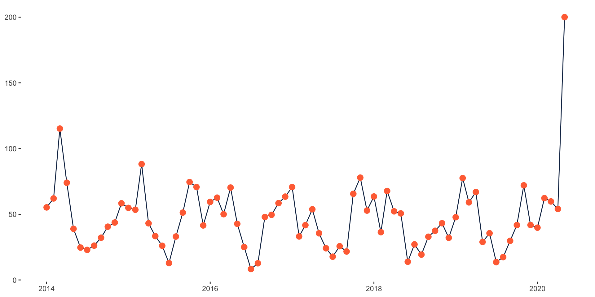
Tags:
comments powered by Disqus