Summer Meals: Census Tract Optimization
Posted on May 28, 2019 | 4 minute readRequired Packages
library(tidyverse)
library(sf)
library(tidycensus)
library(sp)
library(tigris)
Macro Geographies
Durham County Polygon
nc_counties <- counties(state = "37")

durham_county_sf <- nc_counties %>%
  st_as_sf() %>%
  filter(NAME == "Durham")
Durham County Census Tracts
durham_tracts <- tracts(state = "37", county = "063")

durham_tracts_sf <- durham_tracts %>%
  st_as_sf()
Creating Decision Factors
To isolate the census tracts of potential focus, we will first use five different data points from ACS 5-years estimates for Durham County.
- Population Age 3 And Over, Enrolled in School And In Poverty
- Household Received Food Stamps/SNAP in the Past 12 Months
- Median Household Income
- Median Gross Rent as a Percentage of Household Income
- Workers with No Vehicle Available
For factors 1, 2, 3, and 5 we will isolate census tracts by only selecting those that have estimates greater than the overall county median. For factor 4 we will simply select only census tracts that are greater than 30%.
Decision Factor 1
school_age_poverty <- get_acs(geography = "tract", variables = "B14006_003", year = 2017, key = api_key,
                                state = "37", county = "063", geometry = TRUE, summary_var = "B14006_001", survey = "acs5")

pct_poverty <- school_age_poverty %>%
  mutate(pct = round(estimate/summary_est, digits = 2))

poverty_comare <- median(pct_poverty$pct, na.rm = TRUE)

pct_poverty %>%
  filter(pct > poverty_comare) %>%
  ggplot() +
  geom_sf(data = durham_county_sf, fill = "black", color = "black") +
  geom_sf(fill = "red") +
  theme(panel.background = element_blank())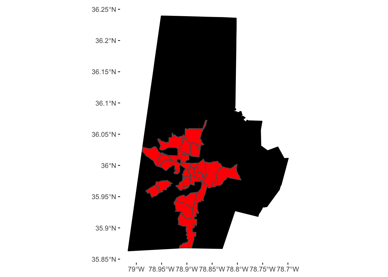
df_1 <- pct_poverty %>%
  filter(pct > poverty_comare)
Decision Factor 2
snap_recepients <- get_acs(geography = "tract", variables = "B22007_002", year = 2017, key = api_key,
                           state = "37", county = "063", geometry = TRUE, summary_var = "B22007_001")

pct_snap <- snap_recepients %>%
  mutate(pct = round(estimate/summary_est, digits = 2))

snap_compare <- median(pct_snap$pct, na.rm = TRUE)

snap_recepients %>%
  filter(estimate > snap_compare) %>%
  ggplot() +
  geom_sf(data = durham_county_sf, fill = "black", color = "black") +
  geom_sf(fill = "red") +
  theme(panel.background = element_blank())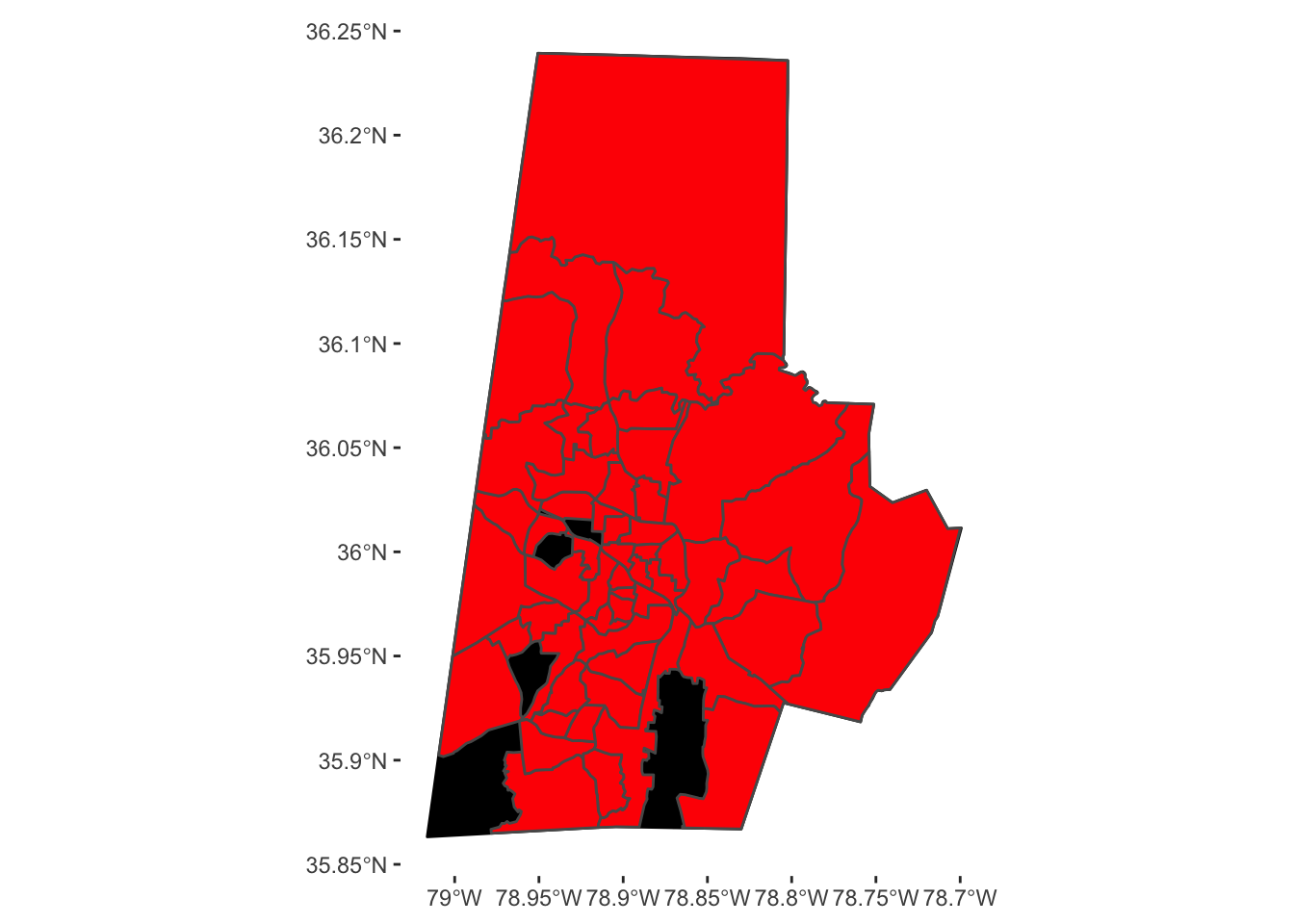
df_2 <- snap_recepients %>%
  filter(estimate > snap_compare)
Decision Factor 3
Pulling median for entire county because you should not compute median on a group of medians. Also, choosing for ACS 1-year estimate for entire county due to accuracy of estimate.
med_household_income <- get_acs(geography = "tract", variables = "B19013_001", year = 2017, key = api_key,
                                state = "37", county = "063", geometry = TRUE)

income_compare <- get_acs(geography = "county", variables = "B19013_001", year = 2017, key = api_key,
                          state = "37", county = "063", survey = "acs1") %>%
  .$estimate

med_household_income %>%
  filter(estimate < income_compare) %>%
  ggplot() +
  geom_sf(data = durham_county_sf, fill = "black", color = "black") +
  geom_sf(fill = "red") +
  theme(panel.background = element_blank())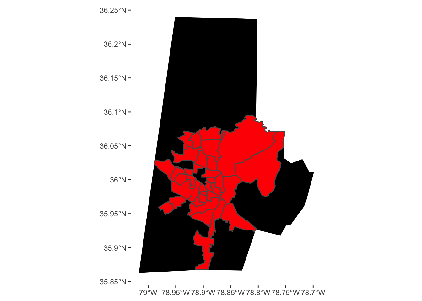
df_3 <- med_household_income %>%
  filter(estimate < income_compare)
Decision Factor 4
gross_rent <- get_acs(geography = "tract", variables = "B25071_001", year = 2017, key = api_key,
                      state = "37", county = "063", geometry = TRUE)

gross_rent %>%
  filter(estimate > 30) %>%
  ggplot() +
  geom_sf(data = durham_county_sf, fill = "black", color = "black") +
  geom_sf(fill = "red") +
  theme(panel.background = element_blank())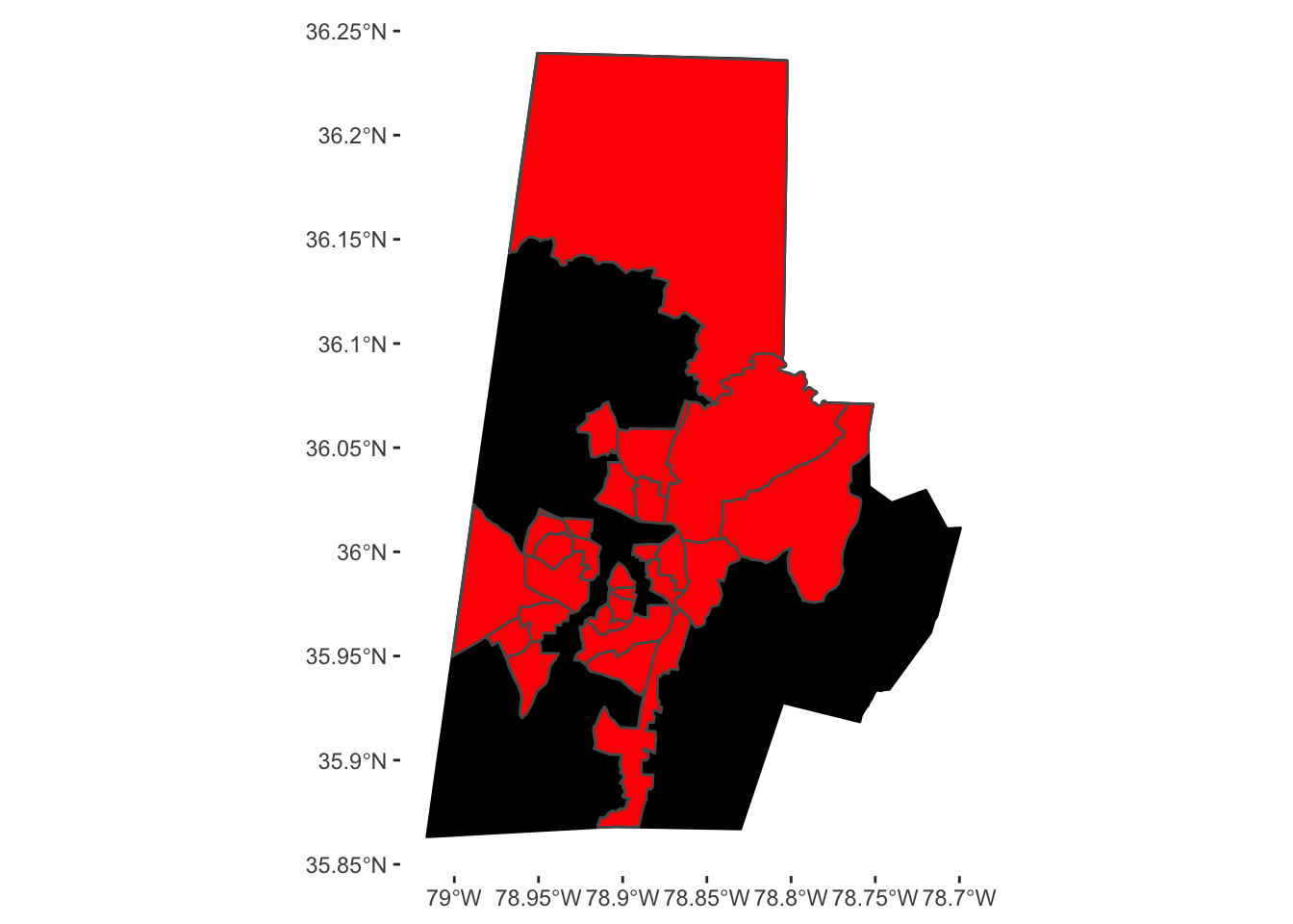
df_4 <- gross_rent %>%
  filter(estimate > 30)
Decision Factor 5
no_vehicle <- get_acs(geography = "tract", variables = "B08014_002", year = 2017, key = api_key,
                      state = "37", county = "063", geometry = TRUE, summary_var = "B08014_001")

pct_no_vehicle <- no_vehicle %>%
  mutate(pct = round(estimate/summary_est, digits = 2))

vehicle_compare <- median(pct_no_vehicle$pct, na.rm = TRUE)

pct_no_vehicle %>%
  filter(pct > vehicle_compare) %>%
  ggplot() +
  geom_sf(data = durham_county_sf, fill = "black", color = "black") +
  geom_sf(fill = "red") +
  theme(panel.background = element_blank())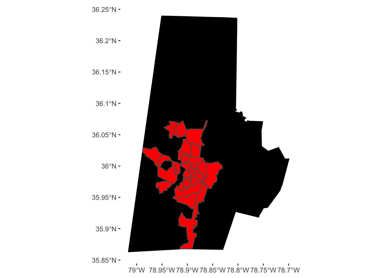
df_5 <- pct_no_vehicle %>%
  filter(pct > vehicle_compare)
Putting It All Together
Filtered Object
This creates an object containing only census tracts that meet all five decision factor criteria
tracts_filt <- durham_tracts_sf %>%
  filter(GEOID %in% df_1$GEOID) %>%
  filter(GEOID %in% df_2$GEOID) %>%
  filter(GEOID %in% df_3$GEOID) %>%
  filter(GEOID %in% df_4$GEOID) %>%
  filter(GEOID %in% df_5$GEOID)
Final Map Visual
tracts_filt %>%
  ggplot() +
  geom_sf(data = durham_tracts_sf, fill = "light grey", color = "black") +
  geom_sf(fill = "red") +
  theme(panel.background = element_blank())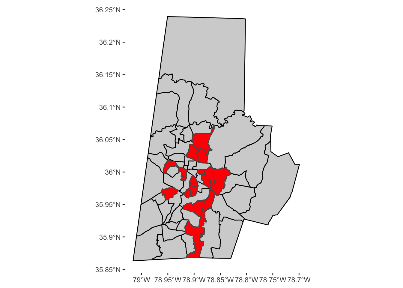
Supplemental Table
tracts_filt %>%
  as_tibble() %>%
  select(1:6) %>%
  kableExtra::kable() %>%
kableExtra::kable_styling()| STATEFP | COUNTYFP | TRACTCE | GEOID | NAME | NAMELSAD |
|---|---|---|---|---|---|
| 37 | 063 | 001002 | 37063001002 | 10.02 | Census Tract 10.02 |
| 37 | 063 | 001301 | 37063001301 | 13.01 | Census Tract 13.01 |
| 37 | 063 | 001303 | 37063001303 | 13.03 | Census Tract 13.03 |
| 37 | 063 | 001304 | 37063001304 | 13.04 | Census Tract 13.04 |
| 37 | 063 | 001502 | 37063001502 | 15.02 | Census Tract 15.02 |
| 37 | 063 | 002015 | 37063002015 | 20.15 | Census Tract 20.15 |
| 37 | 063 | 002026 | 37063002026 | 20.26 | Census Tract 20.26 |
| 37 | 063 | 002300 | 37063002300 | 23 | Census Tract 23 |
| 37 | 063 | 002027 | 37063002027 | 20.27 | Census Tract 20.27 |
| 37 | 063 | 000101 | 37063000101 | 1.01 | Census Tract 1.01 |
| 37 | 063 | 001709 | 37063001709 | 17.09 | Census Tract 17.09 |
| 37 | 063 | 001802 | 37063001802 | 18.02 | Census Tract 18.02 |
| 37 | 063 | 001001 | 37063001001 | 10.01 | Census Tract 10.01 |
| 37 | 063 | 000102 | 37063000102 | 1.02 | Census Tract 1.02 |
| 37 | 063 | 000500 | 37063000500 | 5 | Census Tract 5 |
| 37 | 063 | 000900 | 37063000900 | 9 | Census Tract 9 |
Tags:
comments powered by Disqus