#ELGL19 On Twitter: A Brief Synthesis
Posted on May 24, 2019 | 4 minute readThe Boring Bits
library(tidyverse)
library(lubridate)
library(tidytext)
library(kableExtra)

tweets <- read_rds("data/tweets.rds") %>%
  as_tibble()

f <- function(time) {
  x <- time
  hour(x) <- hour(x)-4
  return(x)
}
24 Hours of Tweets
tweets %>%
  filter(is_retweet == FALSE) %>%
  mutate(created_at = floor_date(created_at, unit = "hour")) %>%
  mutate(created_at = f(created_at)) %>%
  group_by(created_at) %>%
  summarise(tweet_count = n()) %>%
  ungroup() %>%
  arrange(created_at) %>%
  mutate(running_total = cumsum(tweet_count)) %>%
  top_n(24, running_total) %>%
  ggplot(aes(created_at, running_total)) +
  geom_col(fill = "#112E51") +
  geom_label(aes(label = scales::comma(running_total)), nudge_y = -50, size = 2) +
  scale_y_continuous(labels = scales::comma_format()) +
  labs(title = "New Tweets: #ELGL19",
       caption = "Author: Jason Jones, @packpridejones",
       x = NULL, y = NULL) +
  theme(panel.background = element_blank(),
        panel.grid.major.y = element_line(color = "light grey"))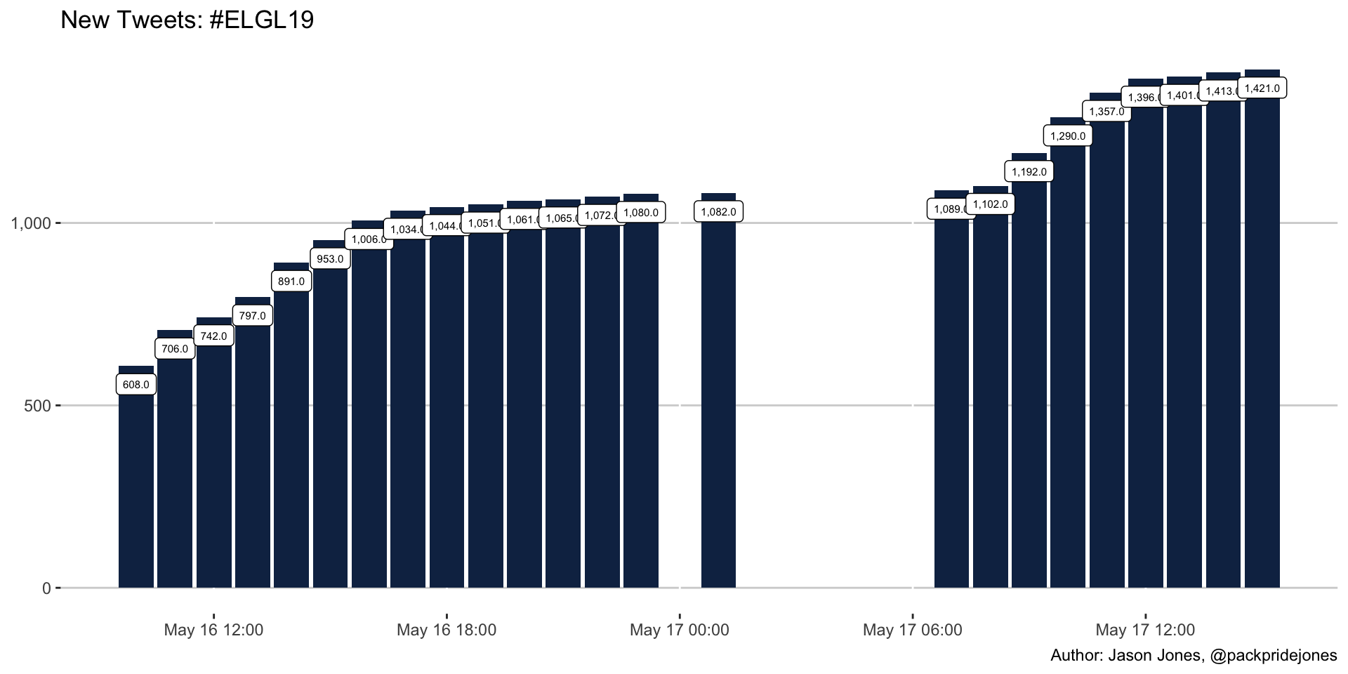
Retweets Are Tweets Too
tweets %>%
  filter(is_retweet == TRUE) %>%
  mutate(created_at = floor_date(created_at, unit = "hour")) %>%
  mutate(created_at = f(created_at)) %>%
  group_by(created_at) %>%
  summarise(tweet_count = n()) %>%
  ungroup() %>%
  arrange(created_at) %>%
  mutate(running_total = cumsum(tweet_count)) %>%
  top_n(24, running_total) %>%
  ggplot(aes(created_at, running_total)) +
  geom_col(fill = "#FF7043") +
  geom_label(aes(label = scales::comma(running_total)), nudge_y = -50, size = 2) +
  scale_y_continuous(labels = scales::comma_format()) +
  labs(title = "Retweets: #ELGL19",
       caption = "Author: Jason Jones, @packpridejones",
       x = NULL, y = NULL) +
  theme(panel.background = element_blank(),
        panel.grid.major.y = element_line(color = "light grey"))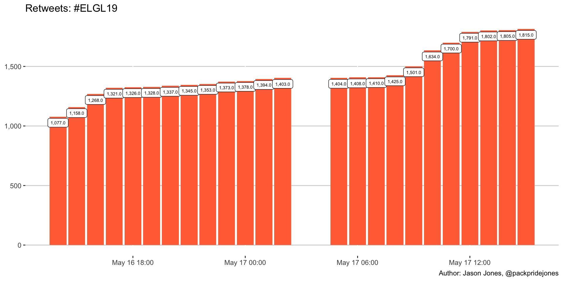
Biggest Fans
Most Original Tweets
tweets %>%
  filter(is_retweet == FALSE) %>%
  group_by(screen_name) %>%
  summarise(tweets = n()) %>%
  arrange(desc(tweets)) %>%
  top_n(10, tweets) %>%
  kable(col.names = c("Twitter ID", "Tweet Count")) %>%
kable_styling()| Twitter ID | Tweet Count |
|---|---|
| kwyatt23 | 134 |
| kowyatt | 97 |
| TheBaconDiaries | 76 |
| acornsandnuts | 54 |
| RealMaggieJones | 54 |
| benkittelson56 | 41 |
| JBStephens1 | 37 |
| Josh_Edwards11 | 35 |
| kimstric | 34 |
| 77ccampbell | 32 |
| BarkmanSusan | 32 |
Cheering Section
Most Retweets
tweets %>%
  filter(is_retweet == TRUE) %>%
  group_by(screen_name) %>%
  summarise(tweets = n()) %>%
  arrange(desc(tweets)) %>%
  top_n(10, tweets) %>%
  kable(col.names = c("Twitter ID", "Retweet Count")) %>%
kable_styling()| Twitter ID | Retweet Count |
|---|---|
| ELGL50 | 243 |
| SEELGL | 125 |
| 77ccampbell | 75 |
| MountainELGL | 67 |
| NWELGL | 58 |
| kowyatt | 56 |
| danwein | 51 |
| acornsandnuts | 45 |
| CALELGL | 38 |
| SWELGL | 37 |
Enough Already!
Top Average Tweet Length
tweets %>%
  filter(is_retweet == FALSE) %>%
  group_by(screen_name) %>%
  summarise(avg_length = mean(display_text_width)) %>%
  top_n(15, avg_length) %>%
  ggplot(aes(reorder(screen_name, avg_length), avg_length)) +
  geom_col(fill = "#0095A8") +
  coord_flip() +
  labs(title = "Average Tweet Length",
       subtitle = "Top 15",
       caption = "Author: Jason Jones, @packpridejones",
       x = NULL, y = NULL) +
  theme(panel.background = element_blank(),
        panel.grid.major.x = element_line(color = "light grey"))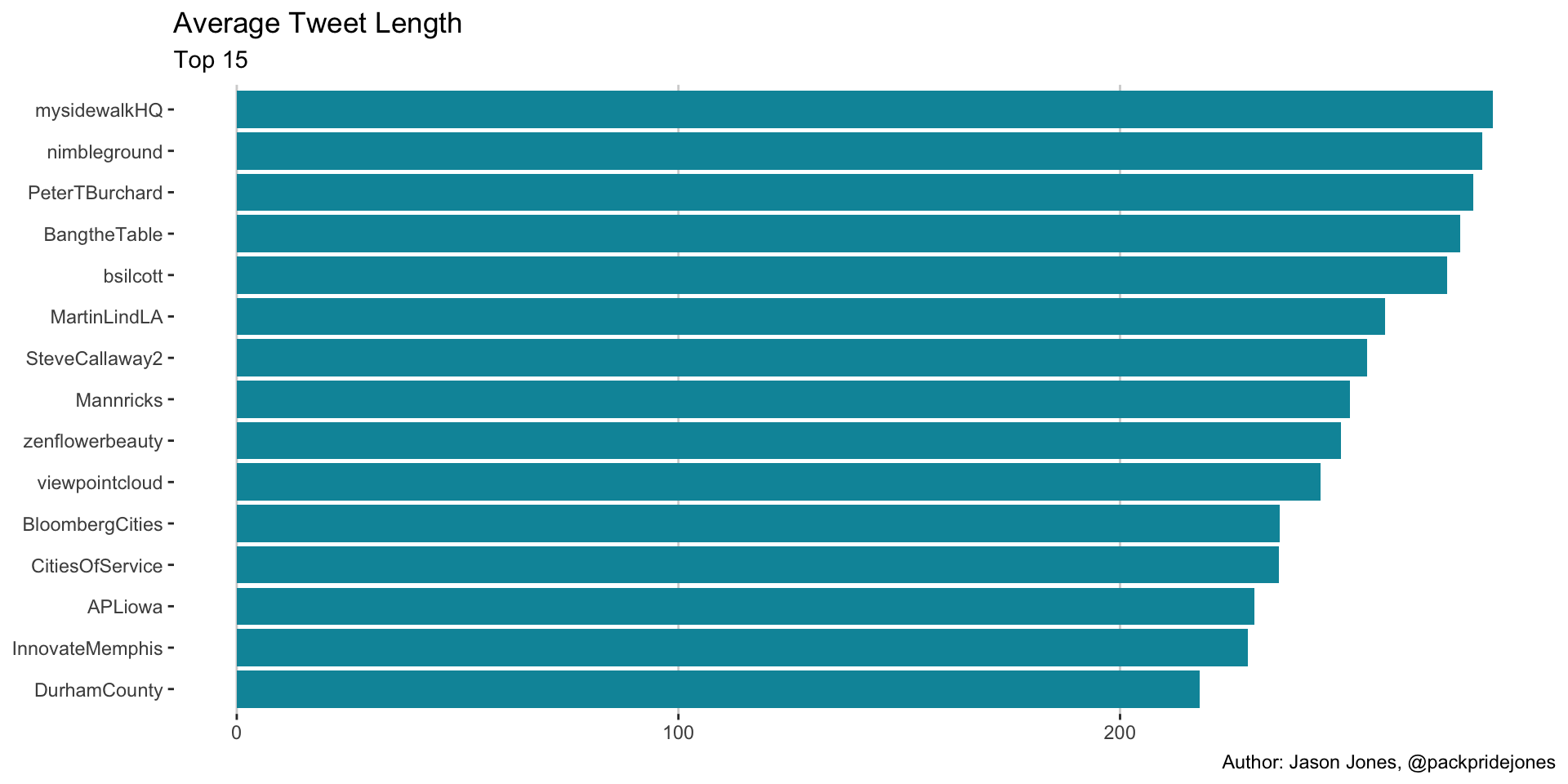
Short and Sweet
tweets %>%
  filter(is_retweet == FALSE) %>%
  group_by(screen_name) %>%
  summarise(avg_length = mean(display_text_width)) %>%
  top_n(-15, avg_length) %>%
  ggplot(aes(reorder(screen_name, desc(avg_length)), avg_length)) +
  geom_col(fill = "#0095A8") +
  coord_flip() +
  labs(title = "Average Tweet Length",
       subtitle = "Lowest 15",
       caption = "Author: Jason Jones, @packpridejones",
       x = NULL, y = NULL) +
  theme(panel.background = element_blank(),
        panel.grid.major.x = element_line(color = "light grey"))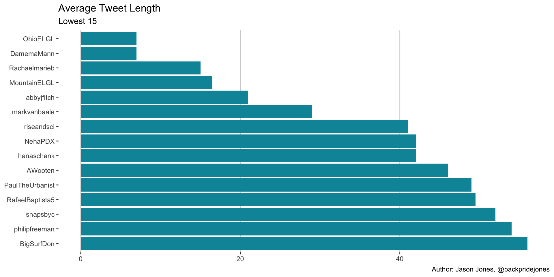
Popular Kids
Who gets the most replies?
tweets %>%
  filter(is.na(reply_to_screen_name) != TRUE) %>%
  group_by(reply_to_screen_name) %>%
  summarise(tweets = n()) %>%
  arrange(desc(tweets)) %>%
  top_n(10, tweets) %>%
  kable(col.names = c("Twitter ID", "Reply Count")) %>%
kable_styling()| Twitter ID | Reply Count |
|---|---|
| kwyatt23 | 21 |
| Josh_Edwards11 | 18 |
| acornsandnuts | 17 |
| TheBaconDiaries | 13 |
| BarkmanSusan | 12 |
| kowyatt | 11 |
| novalsi | 8 |
| marcemars | 7 |
| benkittelson56 | 6 |
| ELGL50 | 6 |
| hanaschank | 6 |
| libraryhillary | 6 |
iPhone or Android?
Twitter tool of choice
tweets %>%
  filter(is_retweet == FALSE) %>%
  group_by(source) %>%
  summarise(Count = n()) %>%
  arrange(desc(Count)) %>%
  top_n(10, Count) %>%
  kable() %>%
kable_styling()| source | Count |
|---|---|
| Twitter for iPhone | 866 |
| Twitter for Android | 353 |
| Twitter Web Client | 99 |
| Twitter Web App | 71 |
| Twitter for iPad | 12 |
| 7 | |
| HubSpot | 4 |
| IFTTT | 2 |
| 2 | |
| Sprout Social | 2 |
Stealing Thunder?
Retweet has more favorites than original tweet
tweets %>%
  filter(favorite_count < retweet_favorite_count) %>%
  group_by(screen_name) %>%
  summarise(thunder_stolen = n()) %>%
  arrange(desc(thunder_stolen)) %>%
  top_n(10, thunder_stolen) %>%
  kable(col.names = c("Screen Name", "Count Of Thunder Steals")) %>%
kable_styling()| Screen Name | Count Of Thunder Steals |
|---|---|
| ELGL50 | 238 |
| SEELGL | 121 |
| 77ccampbell | 75 |
| MountainELGL | 65 |
| NWELGL | 57 |
| kowyatt | 56 |
| danwein | 51 |
| acornsandnuts | 45 |
| CALELGL | 37 |
| MidwestELGL | 36 |
Language Is Important
Scoring Tweets by Language Sentiment
tweets %>%
  filter(created_at > as.POSIXct("2019-05-15 23:59:59")) %>%
  mutate(index = row_number()) %>%
  unnest_tokens("word", text) %>%
  select(index, created_at, screen_name, word) %>%
  anti_join(stop_words) %>%
  mutate(created_at = floor_date(created_at, unit = "hour")) %>%
  mutate(created_at = f(created_at)) %>%
  inner_join(get_sentiments(lexicon = "afinn")) %>%
  group_by(created_at) %>%
  summarise(score = sum(value)) %>%
  ungroup() %>%
  arrange(created_at) %>%
  mutate(sent_flow = cumsum(score)) %>%
  ggplot(aes(created_at, sent_flow)) +
  geom_line() +
  geom_point(color = "#FF7043", size = 3) +
  scale_y_continuous(labels = scales::comma_format()) +
  labs(title = "#ELGL19: Twitter Cumulative Sentiment",
       subtitle = "Y'all Some Positive People!",
       caption = "Author: Jason Jones, @packpridejones",
       x = NULL, y = NULL) +
  theme(panel.background = element_blank(),
        panel.grid.major.y = element_line(color = "light grey"))
Most Used Words
sentiment <- tweets %>%
  filter(created_at > as.POSIXct("2019-05-15 23:59:59")) %>%
  mutate(index = row_number()) %>%
  unnest_tokens("word", text) %>%
  select(index, created_at, screen_name, word) %>%
  anti_join(stop_words) %>%
  mutate(created_at = floor_date(created_at, unit = "hour")) %>%
  mutate(created_at = f(created_at)) %>%
  inner_join(get_sentiments(lexicon = "bing")) %>%
  group_by(word) %>%
  summarise(word_count = n()) %>%
  ungroup()

wordcloud::wordcloud(sentiment$word, sentiment$word_count, colors = c("#0095A8",
                                                                      "#112E51",
                                                                      "#FF7043"))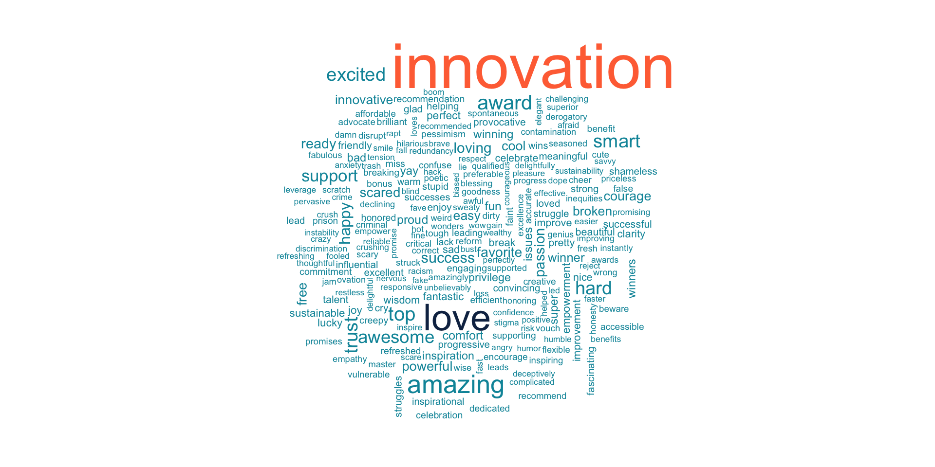
Tags:
comments powered by Disqus